Metrics
Demod implements some metrics that can be used to evaluate the results of the simulations.
Load Metrics
Functions that compute various metrics for load profiles.
A load profile is an array with values equal to the power consumption at various times. Load profiles are by convention in demod arrays of size n_profiles * n_times. Where n_profiles is the number of load profiles and n_times is the number of observations during the time, usually with a constant step size.
-
demod.metrics.loads.total_energy_consumed(load_profiles, step_size=datetime.timedelta(seconds=60))¶ Compute the total energy that was consumed in the profile.
Sums up all the power comsumed by all time to find the total energy. Return the energy in Joules.
- Parameters
load_profiles (numpy.ndarray) – The load profiles, shape = n_profiles * n_times.
step_size (datetime.timedelta) – the step size used in the load_profiles. Defaults to datetime.timedelta(minutes=1).
- Returns
total_energy, The total energy that was consumed in the load profiles (shape = n_profiles).
- Return type
numpy.ndarray
-
demod.metrics.loads.profiles_similarity(simulated_profiles, target_profiles, *args, **kwargs)¶ Compare similarity of each simulated profiles with target profiles.
It uses scipy.cdist to compute the distances. Any args, or kwargs given to this function will be passed to the scipy function.
- Parameters
simulated_profiles (numpy.ndarray) – The simulated profiles. array of shape = (n_profiles_sim, n_times)
target_profiles (numpy.ndarray) – The target profiles for the similarity. array of shape = (n_profiles_target, n_times)
- Returns
similarity_metric, The similarity between the profiles, as an array of shape = (n_profiles_sim, n_profiles_target) where element[i,j] is the comparison of the i-eth simulated profile with the j-eth target profile.
- Return type
numpy.ndarray
-
demod.metrics.loads.profiles_variety(profiles, average=True, *args, **kwargs)¶ Compare variety in the given profiles.
It uses scipy.pdist to compute the distances. Any keyword argument given to this function will be passed to the scipy function.
- Parameters
profiles (numpy.ndarray) – The profiles which should have their variety assessed. array of shape = (n_profiles, n_times)
average (bool) – Whether to average the comparison or to give the distance from each profile to every other
- Returns
variety_metric, The variety between the profiles, as an array of Shape = (n_profiles, n_profiles) where element[i,j] is the comparison of the i-eth profile with the j-eth profile.
- Return type
Union[numpy.ndarray, float]
-
demod.metrics.loads.diversity_factor(profiles)¶ Compute the diversity factor for the given load profiles.
The diversity factor is the ratio of the sum of the individual non-coincident maximum loads to the maximum demand of the aggregated loads. More on wiki .
- Parameters
profiles (numpy.ndarray) – The load profiles. Shape = (n_profiles, n_times).
-
demod.metrics.loads.coincidence_factor(profiles)¶ Compute the simultaneity factor for the given load profiles.
The simultaneity factor is the inverse of the
diversity_factor().- Parameters
profiles (numpy.ndarray) – The load profiles. Shape = (n_profiles, n_times).
-
demod.metrics.loads.simultaneity_factor(profiles)¶ Compute the simultaneity factor for the given load profiles.
The simultaneity factor is the same as the coincidence factor.
coincidence_factor().- Parameters
profiles (numpy.ndarray) – The load profiles. Shape = (n_profiles, n_times).
-
demod.metrics.loads.cumulative_changes_in_demand(profiles, bins=100, normalize=True, bin_edges=None)¶ Return the distribution of the changed in demand.
Can be used as a measure of the ‘spikiness’ or ‘volatility’ of the loads. The distribution correspond to how often the load varies during the days.
- Parameters
profiles (numpy.ndarray) – The load profiles which are used to compute the demand. shape = (n_profiles, n_times).
bins (int) – The number of intervals to used for the cumulative distribution.
normalize (bool) – Whether to normalize the demand by the maximum demand.
bin_edges (Optional[numpy.ndarray]) – If specified, these edges will be used instead. When using this, make sure that if kwarg
normalizeis True, the edges scale from 0 to 1.
- Returns
cdf, array with the values of the histogram. The value of cdf[i] corespond to the values between bin_edges[i] and bin_edges[i+1].
bin_edges, array of dtype float Return the bin edges (length(hist)+1).
- Return type
Tuple[numpy.ndarray, numpy.ndarray]
-
demod.metrics.loads.time_coincident_demand(profiles)¶ Return the time coincident demand for the given profiles.
The maximum demand per household during the whole time.
For large number of profiles, this metric is equal to the after diversity maximum demand (ADMD) , as it is is “the maximum demand, per customer, as the number of customers connected to the network approaches infinity.” [McQueen2004]
- Parameters
profiles (numpy.ndarray) – The load profiles which are used to compute the demand. shape = (n_profiles, n_times).
- Return type
float
-
demod.metrics.loads.load_duration(profiles, loads=None)¶ Compute the load duration of the given profiles.
The outputs can be used to build the load duration curve .
n_loads, the number of load thresholds returned is either given by
loadsor by the number of unique loads in profiles- Parameters
profiles (numpy.ndarray) – The load profiles which are used to compute the demand. shape = (n_profiles, n_times).
loads (Optional[numpy.ndarray]) – The different loads thresholds at which the durations should be computed. size=n_loads
- Returns
loads, Array of the loads (sorted), size = (n_loads)
durations, The durations correponding to the loads (in steps). size = (n_profiles, n_loads)
- Return type
Tuple[numpy.ndarray, numpy.ndarray]
States Metrics
Different metrics to help using states patterns.
A state is a discrete value, that can change during a time period. A state pattern records the value of the state over the time period. States represent a number of different states patterns on the same time period. In demod states are numpy arrays containing the states patterns, and is of shape n_patterns * n_times.
-
demod.metrics.states.get_states_durations(states)¶ Get the durations from the states matrix given as input.
Will merge end and start of the diaries to compute the duration, if the starting and ending states or the same.
- Parameters
states (numpy.ndarray) – States patterns array
- Returns
durations, a ndarray with the durations of each states
corresponding_states, a ndarray with the labels of the states for each duration
- Return type
Tuple[numpy.ndarray, numpy.ndarray]
Note
The position of the durations in the returned arrays does not correspond to how they happened during time.
-
demod.metrics.states.get_durations_by_states(states)¶ Return a dict of all the durations depending on the states.
- Parameters
states (ndarray(int, size=(n_households, n_times))) – The matrix of the states for the housholds at all the times
- Returns
durations_dict, dictionary where you can access by giving the state and recieve an array containing all the durations for this state
- Return type
Dict[Any, numpy.ndarray]
-
demod.metrics.states.count(array)¶ Count the number of elements in the input array.
Usefull to have a quick view of the values present in the array.
- Parameters
array (numpy.ndarray) – the input array to be counted
- Returns
A list of tuples contanining the elements and their counts
- Return type
List[Tuple[Any, int]]
-
demod.metrics.states.graph_metrics(states)¶ Compute and return 4 graph metrics for given States patterns.
These metrics are an attempt to implement graph metrics as proposed by [McKenna2020]. The following description of the metrics comes from the paper.
- Parameters
states (numpy.ndarray) – An array containing the states for which we want to compute the graph metrics
- Returns
network_size, Refers to the number of unique nodes in a network. For states sequence networks the size describes the number of unique observations of states and the time they occur at. A larger network is one where more states were observed and gives an indication of the diversity of states that occurred.
network_density, The fraction of the total maximum number of possible connections that are actually observed in the network. Network density is calculated by counting the number of unique edges observed in the network and dividing it by this maximum. It is a measure of the diversity of sequences present in the network. A denser network is one where there are more alternative pathways between time periods by different people.
centrality, Refers to how dominant certain pathways or nodes are within a network. Central states nodes are those that are highly connected to others. Central connections or edges are those that appear in many individual sequences i.e. those with high ‘weight’. There are multiple ways of calculating centrality, here we use edge weight as a measure of (path) centrality and compute the mean and standard deviation of the distribution of edge weights for each network.
homophily, Refers to the likelihood that a node is connected to another node of the same type. Here this refers to when a state in one time period is connected to the same state in an adjacent time period. It is a measure of the extent to which states tend to endure in unbroken lasting sequences. A simple measure of homophily used here is the proportion of times a state in one time period is followed by the same state in the following time period. This is calculated for each sequence and the mean of the distribution is taken as the measure of the homophily of the network.
- Return type
Tuple[numpy.ndarray, numpy.ndarray, numpy.ndarray, numpy.ndarray]
-
demod.metrics.states.sparsity(tpm)¶ Return the proportion of 0 elements in the TPMs.
= 0. If all the elements are given= 1. If the tpms are only 0- Parameters
tpm (numpy.ndarray) – The transition probability matrices.
-
demod.metrics.states.average_state_metric(simulated_state, measured_state, average_over_timestep=True)¶ Determine the average per time step state error.
This is a generalization of the Average occupancy metric from [Flett2016] .
It determines the average per time step state error between simulated data and real data from the TOU surveys, quantifying the quality of the calibration of the simulation.
It is defined as
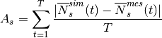
where
 are the average number of subjects in state
 at time
  .
.Two means of analysis are possible with this metric.
It can be used to calculate the prediction for the average per time step results of multiple profiles generated using the model. This determines how effectively the model converges to the population average.
It can be used to calculate the prediction error for each individual profile. The mean of this error can be used to determine how effectively individual profiles replicate the input data.
- Parameters
simulated_state (numpy.ndarray) – The state that have been simulated. Array of shape = (n_subjects/n_households, n_times). The value should be the number of person performing the states at each time of the diaries.
measured_state (numpy.ndarray) – The state that where measured. Same array as simulated_state. n_times must be the same as simulated_state, but n_subjects/n_households can be different.
average_over_timestep (bool) – whether to average the result over the time steps. If false, will return an array of shape = (n_times).
- Returns
average_state_error, The average state error between simulated_state and measured_state.
- Return type
Union[List[float], float]
-
demod.metrics.states.state_duration_distribution_metric(simulated_state, measured_state, average_over_timestep=True)¶ Compare the difference in state durations.
This is a generalization of the State duration distribution metric from [Flett2016] . This metric is commonly known as the Earth Movers Distance: a commonly used quantitative histogram similarity measure where the bin values are not independent and cross-bin analysis is required.
The ‘error’ is the sum ofthe absolute difference between the simulated and mesured data CDFs at each duration value for each state.
It is defined as
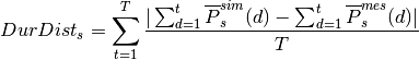
where
 is the probability of a state duration of
 for state .
Note that this metric weights the same, erorrs in durations probs that are unlikely to happen as errors in duration probs that are very likely.
It could be nice to do a weighted average instead, that uses the weight according to the pdf ?
- Parameters
simulated_state (numpy.ndarray) – The state that have been simulated. Array of shape = (n_subjects/n_households, n_times). The value should be the number of person performing the states at each time of the diaries.
measured_state (numpy.ndarray) – The state that where measured. Same array as simulated_state. n_times must be the same as simulated_state, but n_subjects/n_households can be different.
average_over_timestep (bool) – whether to average the cdf over the time steps. If false, will return an array of shape = (n_times) being the absolute difference of each cdf value.
- Returns
duration_distribution, The state duration distribution difference metric.
- Return type
Dict[Any, Union[List[float], float]]
-
demod.metrics.states.levenshtein_edit_distance(profile1, profile2)¶ Compute the Levenshtein Edit Distance Method (LEDM) between 2 profiles.
Can be used to compare the similarity between two discrete profiles, as suggested by [Flett2016] .
You can use this distance combined with
demod.metrics.loads.profiles_similarity()to compare many different profiles, by passing levenshtein_edit_distance as an arg of profiles_similarity().Warning
Currently this is only implemented if the profiles contains single digit integers ranging from 0 to 10 (not included).
Warning
Requires an extra library to be installed https://pypi.org/project/python-Levenshtein/
- Parameters
profile1 (numpy.ndarray) – Two profiles given as arrays of size 1. They must be integers.
profile2 (numpy.ndarray) – Two profiles given as arrays of size 1. They must be integers.
Following description comes from [Flett2016]
This LEDM method is used to quantify the dissimilarity between two strings by quantifying the measures needed to transform one into the other. In the LEDM a ‘cost’ of 1 is assigned for each edit (insertions, deletions, and replacements) required in the trans- formation. For example, transforming 110111 to 001011 would require a minimum edit of a replacement of the first digit, deletion of the second, and insertion of the last digit – a total cost of 3. The approach can therefore be applied when comparing two numerical profiles. When two profiles are compared, for clarity,the total ‘cost’ is converted from a per-time step to an hour equivalent by dividing the result by the number of time steps per hour. The metric can be used in two ways.
It can be used to compare the output profiles with the input dataset. The smallest cost per profile, representative of the closest match, is determined and an average calculated across all mod- elled days. This is a measure of the average similarity between generated profiles and the closest real profile.
Each profile in either the input dataset or model output dataset can be compared with other profiles in the same dataset quantifying the behavioural similarity within and between each dataset.
Error Metrics
Error metrics functions.
Implementation of different error metrics.
-
demod.metrics.errors.RMSE(x1, x2)¶ Compute the Root Mean Squared error between x1 and x2.
- Parameters
x1 (numpy.ndarray) – array 1
x2 (numpy.ndarray) – array 2, must have the same shape as x1
- Returns
The RMSE between x1 and x2.
- Return type
rmse